LOOKUP (Array) Formula in Excel

 

What Does It Do ?

This function looks for a piece of information in a list, and then picks an item from the last cell in the adjacent row or column.

It always picks the data from the end of the row or column, so it is no good if you need to pick data from part way across a list, (use VLOOKUP or HLOOKUP).

The way in which the function decides whether to pick from the row or column is based on the size of the table.

If the table has more rows than columns :

The function will look down the left most column trying to find a match for the piece of information you asked it to look for.

When a match is found, the function will look across to the right most column to pick the last entry on the row.

If the table has the same amount of rows and columns :

The function will look down the left most column and work in just the same way as if the table had more rows than columns, as in the description above.

If the table has more columns than rows :

The function will look across the top row trying to find a match for the piece of information you have asked it to look for.

When a match is found, the function will then look down to the bottom cell of the column to pick the last entry of the column.

Syntax

=LOOKUP(WhatToLookFor,RangeToLookIn)

The WhatToLookFor should be a single item.

The RangeToLook in can be either horizontal or vertical.

Be careful not to include unnecessary heading in the range as these will cause errors.

Formatting

No special formatting is needed.

Problems

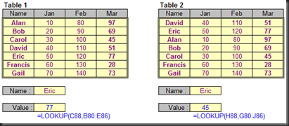
The list of information to be looked through must be sorted in ascending order, otherwise errors will occur, either as #N/A or incorrect results.

Table 1 shows the Name column sorted alphabetically, the results of using =LOOKUP() will be correct.

Table 2 shows the same data, but not sorted. Sometimes the results will be correct, but other times the result will be an #N/A error or incorrect figure.